Simulations and sessions in OpenCell
About this tutorial
In this tutorial we're going to demonstrate some of the more advanced simulation functionality of OpenCell, and show how to set up a session. A OpenCell session is a configuration file that allows a user to set up the interface to display a set of simulation results in a particular way. Sessions are particularly useful for demonstration purposes such as getting a model to automatically reproduce figures from a publication.
This tutorial assumes basic knowledge of CellML and usage of OpenCell as described in the OpenCell model building tutorial.
N.B. We use OpenCell 0.6 in this tutorial. The tutorial will be updated with successive versions of OpenCell with the caveat that there may or may not be some delay in this process.
Downloading a model from the CellML Model Repository
The first thing we'll do is download a model from the CellML Model Repository. The Repository contains hundreds of freely available curated CellML descriptions of models.
Point your browser to http://models.cellml.org/ and click on Exposures. Take a look through the listing to get an idea of the kinds of models that CellML is typically used to describe. Models of cellular systems form the majority of the listing, although CellML is purposefully generic and is increasingly being used to describe other models, including those of non-biological systems.
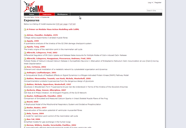
CellML Model Repository model listing
The model we're going to work with is a simple, well known circadian rhythm model by Albert Goldbeter.
Scroll down to: Goldbeter, 1995 and click on the link. This will take you to a page with some documentation and a diagram of the model, and download links at the top. Click Download and save the model to your hard drive. Also click the Solve using OpenCell Session File link and save that to your hard drive as well.
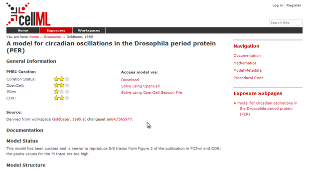
Goldbeter 1995 model description page
Simulating and graphing model solution
To start off, load OpenCell and open the CellML model you just downloaded. You might notice that there isn't much space for the graph window - if you want you can click the partitions and drag them around to set the interface up how you like it. Try closing the left-most pane by dragging the left-hand slider all the way to the edge of the screen.
If you look at the integration pane (marked by red border in screenshot below,) you'll notice that the model integration defaults are set so that the model gets simulated for 75 hours. If you change these values and then resave the model, OpenCell will save these values to the model's metadata, and they will be the default values next time you load the model.
The three basic integrator settings are the point density, the end time point and the step size. If you have a fairly stiff (large changes in values over a small amount of time,) it is a good idea to set the point density relatively high and the step size to a fairly small number. The value for point density is relative to the time end point - so a model with a point density of 1000 and a time end point of 10 hours would have a higher point density than a model with a time end point of 100 hours. The default values for the Goldbeter 95 model we are looking at are set to a moderate setting. There are also more integrator settings you can play with if you desire under the Advanced settings tab.
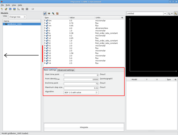
OpenCell integration interface
Integrate the model and make a few traces. If we want to reproduce some of the graphs from the original publication we can make traces against time (in the environment component) for:
| Component | Variable |
|---|---|
| M | M |
| P0 | P0 |
| P1 | P1 |
| P2 | P2 |
| Pt | Pt |
| PN | PN |
This will allow us to reproduce Fig. 2 from the publication.
Note that the trace type is set to dots in the screenshot below to create emphasis. If the point density is high enough, the dots merge into a thick line.
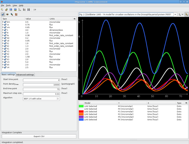
Fig 2. from Goldbeter 1995 paper
Setting up a OpenCell session
Now we're going to have a look at an example session before we make our own one. So open the goldbeter_1995_session1.xml session file that you just downloaded in OpenCell. OpenCell will load up the session. OpenCell now shows us three display panes on the right: a graph window, a key and a diagram of the model - the same one we saw in the model documentation. You'll also notice that the model tree pane on the left is not present and the other panes are resized. As mentioned before, we can customise how we see the OpenCell interface - these customisations can be saved in a session.
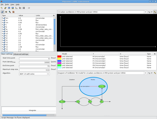
Goldbeter 1995 session with SVG diagram
This particular session is set up so that the species shown can be clicked on to show the concentration / time traces in the graph window above. This is an advanced session feature which is shown for demontration purposes only in this tutorial.
Now, let's create our own session.
Close OpenCell and reload it again, and open the Goldbeter 95 model (not the session, just the *.cellml model.) Integrate the model and then grab the left-most slider with your mouse and drag it to the left of the screen - that pane should snap shut, giving us a bit of space to work with. Now resize the middle pane in a similar manner so that the text within it fits snugly. We're going to get OpenCell to display three graph windows, so under the View menu at the top, select Three (3) graphs.
Next to the title of each graph window (currently 'Untitled') you should see a key icon - click it for each of the graph windows. Create traces for M and P0 in the first window, P1 and P2 in the second, and Pt and PN in the third, all vs time. OpenCell automatically selects colours for the traces from a palette so if you don't like the colour of a trace, click on the coloured box and select a new one. Give your graphs some appropriate names, and if you wish, close the key windows by clicking the key icon and. You can also adjust the relative sizes of the graph windows using the sliders.
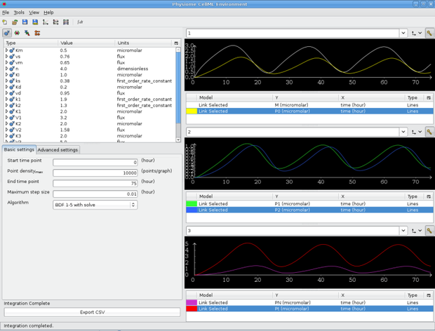 New tutorial session

New tutorial session
Now, let's save the session. In the File menu, select Export session and save the session as goldbeter95_session.xml. The next part is important - you also need to save the CellML file, so hit Save in the file menu. This is because creating a session adds ID tags in the CellML file to the variables we want to graph - we need to save the file so that the session can then reference them.
Try reloading OpenCell and opening our new session file using File > Open. OpenCell should rearrange itself as it was when we saved the session, and if you integrate the model, you should see the graphs that you set up.

