Part 1

The easiest way to get started with CellML is to build and run a model in Cellular Open Resource (COR), an open source tool which provides the ability to write a model in a pascal-esque language, which it then translates into CellML. COR is available here: http://cor.physiol.ox.ac.uk/Download/

Downloaded, installed and run, it looks like this:

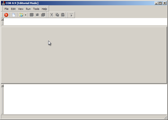
To open a new model click the icon circled in red above.

Model Structure

Let's begin with defining a simple model with some equations in a single component.

COR will have populated the new model with the following:

def model MyModel1 as
enddef;

You can change the 'MyModel1' to something else, for example 'tutorial1', and that becomes the name of your model. You write the rest of your model between the def and enddef statements.

All Cellml equations occur within components, which allows the models to be modular. In the case of this simple model we will construct a single component to provide a location for our example equations:

def model MyModel1 as
def comp firstComponent as
enddef;
enddef;

Here I've added a component called 'firstComponent'. Components contain variables and equations.

Model Variables and Equations

Let's suppose I want to express the following reaction:

Using Mass Action kinetics we might model this as:

For this we need 3 variables; one each for A, B and C. We also define two parameters k_f and k_b which will be included as two more variables. We define an additional variable to hold the flux J. Finally we define a last variable 't' to give the model a sense of time.

Here are some basic variable definitions made between the def comp and it's corresponding enddef statement:

var t: second;
var A: uM {init: 2};
var B: uM {init: 3};
var C: uM {init: 0};
var kf: per_uM_per_second {init: 0.15};
var kb: per_second {init: 0.5};
var J: uM_per_second;

Notice I have provided units and, as appropriate, some initial values for the species A, B and C. I have also provided values for the two reaction rate constants.

We define the equations above in the following way:

J = kf * A * B - kb * C;
ode(A,t) = -J;
ode(B,t) = -J;
ode(C,t) = J;

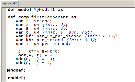
The entire code for this model therefore looks like this:

Model Units

In its current state this model is not valid CellML and it won't run because we haven't defined what our units mean. There are several base units 'built-into' COR (such as 'second') which roughly correlate to SI standard units, but otherwise we are expected to define our units. This may add a bit of work to the creation of a basic model but it provides us with a great flexibility and it also allows tools such as COR to check that our model equations have consistent units. This can help us to find mistakes in our model before it is published and/or someone else does!

Units are defined by units statements, and can appear anywhere between def model and the associated enddef tags. We generally place such statements at the top of the model definition.

As an example, here we include a new unit 'per_second', defined as being 1 over a second:

def unit per_second from
    unit second {expo: -1};
enddef;

Notice the use of the 'expo' keyword. Another keyword is 'prefix' that allows us to define SI scalings of units, such as micromolar:

def unit uM from
    unit mole {pref: micro};
    unit liter {expo: -1};
enddef;

This says that a micromolar (uM) is a micromole, divided by a liter.

We can define new complex units in terms of other units that we have previously defined. For example:

def unit uM_per_second from
    unit uM;
    unit per_second;
enddef;

Which is defined in terms of the previous two units.

See the specifications for a list of available units, and further down in that document for a list of supported prefixes.

Can you define the units for 'per_uM_per_second'?

Completed Model

Once all the units are defined, we have a complete, runnable CellML file. Rendered in COR, it looks like this:

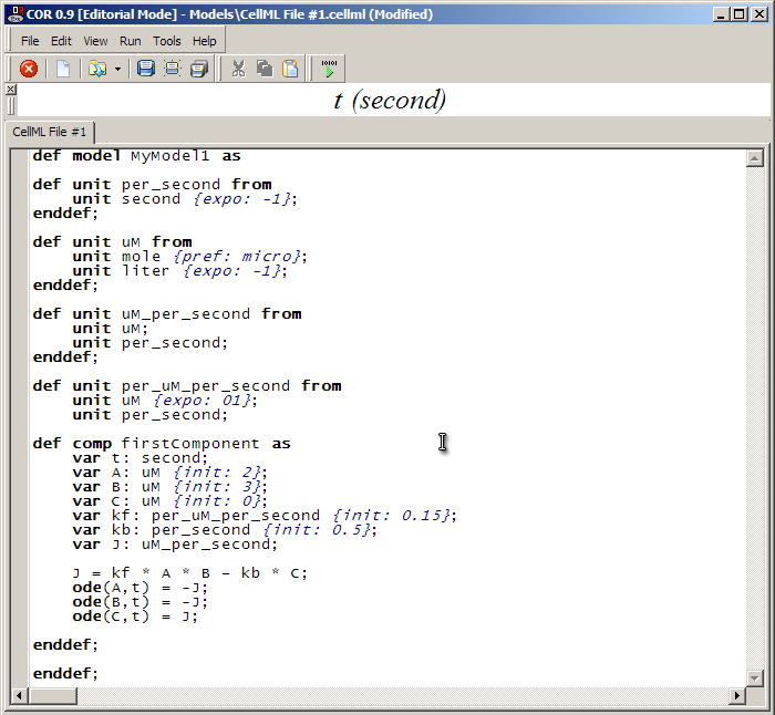
You will be able to save your model to disk (such as the Desktop) by clicking on the 'Save' icon in the toolbar and filling out the dialog box.

To run the model, click on the green play button as circled above. This takes us to the simulation screen of COR.

Simulating the Model

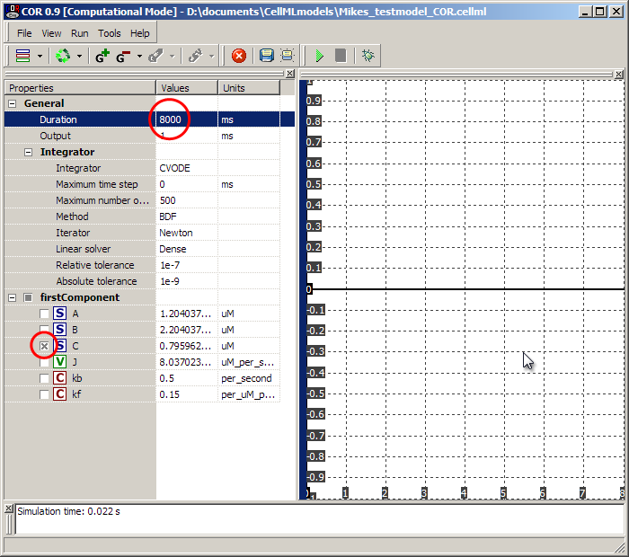
In the simulation screen, set the 'Duration' to 8000ms as shown, and select the 'C' species. Then hit the green play button in the toolbar. The graph on the right should populate with a growth curve for the 'C' species as it is made from A and B according to the maths we defined.

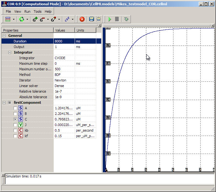
The actual values of the species are given on the left. You could run the model for a further 8000ms (or any duration) by clicking the play button again - it will run from the last simulated point. To get back to the 'beginning' of the simulation, click on the 'recycle' arrows in the toolbar. You can also experiment further by selecting more variables on the left, and with the CSV option in the toolbar, it is a good way to get time-course data from the model into something that can be analysed (such as your favourite spreadsheet).

To return to the model editing window from the simulation screen, hit the red stop sign button in the toolbar.

COR Limitations, CellML 1.1 models and PCEnv

At the time of writing, COR is limited to CellML 1.0 models, which means that one cannot produce multi-file CellML 1.1 models using the importCellML keyword. Personally, I tend to develop my models in COR in one big file, then edit the text file to produce a set of network of imported CellML files (as per CellML v1.1). COR cannot run CellML 1.1 models, so once my models are at that stage I run them in OpenCell, another freely available, open source tool which can be used for building and running CellML models. This tool will be covered in a little more detail in Tutorial 3.

Therefore it is still useful and occasionally necessary to understand the CellML itself, irrespective of the more human-readable language offered by COR.

The CellML Language

Open the saved CellML file in your favourite text editor (hint - Notepad++ is a nice one to use under Windows!). Here we compare some of the COR-language constructs with the generated CellML.

After some comments and header information the model will begin with a model definition tag like this:

<model
    name="MyModel1"
    cmeta:id="MyModel1"
    xmlns="http://www.cellml.org/cellml/1.0#"
    xmlns:cellml="http://www.cellml.org/cellml/1.0#"
    xmlns:cmeta="http://www.cellml.org/metadata/1.0#">

For now this detail can be ignored, it will only be edited if we later decide to upgrade this CellML 1.0 model to a CellML 1.1 model (using modular imports) or extend the CellML we are using in some way (such as adding metadata other than that supported by the above 'cmeta' namespace).

The units definitions come next, which look something like this:

<units xmlns="http://www.cellml.org/cellml/1.0#" name="uM">
  <unit units="mole" prefix="micro"/>
  <unit units="liter" exponent="-1"/>
</units>

Compare these tags to the COR definition above, and note the correspondence.

After the units comes the component we defined:

<component xmlns="http://www.cellml.org/cellml/1.0#" name="firstComponent">

Which contains variables:

<variable name="kf" units="per_uM_per_second" initial_value="0.15"/>

All of which should be recognisable given the work we did in COR above.

After the variables of a component come the mathematics defining the equations. CellML uses a subset of MathML to define the relationships between variables in the models.

Like the rest of CellML, MathML is an XML-based language. All MathML within a CellML document is enclosed in <mathml> tags:

<math xmlns="http://www.w3.org/1998/Math/MathML">
</math>

MathML uses polish notation. This means that operators come before their operands. This makes it easy for the computer to process, but a little harder at first for people to read.

The first chunk of CellML is:

<apply>
  <eq/>
  <ci>J</ci>
  <apply>
    <minus/>
    <apply>
      <times/>
      <ci>kf</ci>
      <ci>A</ci>
      <ci>B</ci>
    </apply>
    <apply>
      <times/>
      <ci>kb</ci>
      <ci>C</ci>
    </apply>
  </apply>
</apply>

The <apply> tag means to apply an operator to something. The first operator is <eq> which means '='. This is applied to J, and another apply which means the second operand of '=' is itself composed of at least one operator and operand set.

If you think of 'apply' tags as being like brackets, you could rewrite the above CellML in the following way:

= J (- (* kf A B) (* kb C) )

In English, it is sometimes easier to find the innermost level of bracket and work out. For example, at the bottom level we have kb* C and kf * A * B ('*' can take multiple operands, which it multiplies together). These two elements are being subtracted, which overall gives us: (kf * A * B) - (kb * C). Unlike '*', the order for '-' is important, here the second operand is always subtracted from the first operand. This is the second operand of '=', the first operand of which is J. In English this means

J = (kf * A * B) - (kb * C)

. Here we have our expression for the flux J described above.

The next equation is:

<apply>
  <eq/>
  <apply>
    <diff/>
    <bvar>
      <ci>t</ci>
    </bvar>
    <ci>A</ci>
  </apply>
  <apply>
    <minus/>
    <ci>J</ci>
  </apply>
</apply>

<diff>means a differential equation, and <bvar>defines the 'bound variable', in this case t (time). This cellml could be rewritten as

= (d (by t) A) (- J)

The first operand of '=' goes to the left hand side in English, yielding

dA/dt = -J

For details on what operators and constructs of MathML are supported by CellML, please see the CellML specification (at the time of writing, the best reference for this is in the specifications).

This model finishes with closing the component and model (since there is only one component) with the following XML tags:

</component>
</model>

This completes Tutorial 1.

Tutorial 2 will introduce a second component and the concept of variable interfaces and connections to allow communication between components.