Part 2
Let's imagine that the biological system we are modelling produces a voltage that is dependent on the concentration of the 'C' species above. Perhaps 'C' activates a set of ion transporters which then alter the voltage across the cell membrane.
Assume that the relationship between 'C' and voltage ('V') was derived empirically as follows:

Since we don't know the biophysical basis of this relationship, we decide to model this in another component, to separate the biophysical activities modelled in Tutorial 1 from these 'lumped' formulations.
Adding a Second Component
The second component is defined in a similar manner to the first component:
    def comp secondComponent as
    enddef;
We define variables and equations in order to express the equation for V defined above:
    var C: uM {pub: in};
    var V: millivolt;
    V = 1{millivolt}/(1{dimensionless}+exp((C+1.6{uM})/-1.42{uM}));
There are some new constructs here. Firstly the variable 'C' defined in this component will have a public interface of 'in'. That means it gets its value from some other component.
Secondly, the expression for V has some units embedded in the equation. This is necessary when you want to put constant values in - CellML solvers need to know what units those constants have.
Notice also we are working with millivolts, which need to be defined like so:
    def unit millivolt from
        unit volt {pref: milli};
    enddef;
'volt' is a predefined unit which we have prefixed with 'milli'.
We need to connect the two components together, by feeding the value of 'C' defined in the first component to the value of 'C' in the second component. We do this with a map statement:
    def map between firstComponent and secondComponent for
        vars C and C;
    enddef;
Note that in the second component we could have called 'C' anything we liked, and simply changed the name referenced in the map statement.
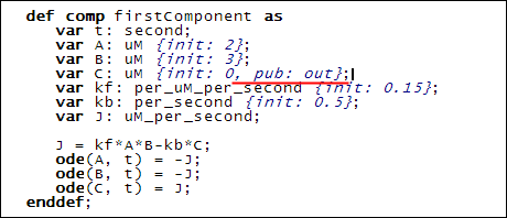
Finally, since 'C' from 'firstComponent' feeds into 'C' from the 'secondComponent', we give 'C' in the 'firstComponent' a public interface of 'out':

This addition is shown underlined in red above.
Simulating the Model
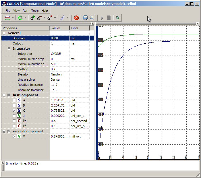
Pushing the 'play' button we can simulate the new model thus:

Here we see 'C' and 'V' climbing over a period of 7-8 seconds.
The CellML Language
The public interface elements are implemented as attributes on the <variable> tag in CellML:
<variable name="C" units="uM" initial_value="0" public_interface="out"/>
from the 'firstComponent', and
<variable name="C" units="uM" public_interface="in"/>
from the 'secondComponent'.
The units for numerical constants in CellML are implemented using <cn> tags:
<cn cellml:units="millivolt">1</cn>
whereas variables in equations are included using <ci> tags as in Tutorial 1:
<ci>C</ci>
Variable mapping between components is achieved using the following construct:
  <connection xmlns="http://www.cellml.org/cellml/1.0#">
    <map_components component_1="firstComponent" component_2="secondComponent"/>
    <map_variables variable_1="C" variable_2="C"/>
  </connection>
Additional <map_variables> tags can be added to <connection> tags which is necessary if you are linking multiple variables between two components. Every component pair that you are linking between should have its own <connection> tag.
You can also define containment and encapsulationhierarchies of components, which collectively are termed groups, but these are only useful in specific situations. You can read about them in the specifications if you are interested.
On a related note, you can also read about public versus private interfaces on variables in the specifications.
This completes Tutorial 2. Tutorial 3 will turn this two-component model into a CellML 1.1 model, where the components are in separate files, one importing the other.

